Image made using the COMSOL Multiphysics® software and is provided courtesy of COMSOL.
Comparison of the flow field in a 2D approximation with the 3D model of a baffled, turbulent reactor.
The CFD Module is a numerical simulation platform for computational fluid dynamics (CFD) that accurately describes your fluid flow processes and engineering designs. Using the CFD Module, you can model most aspects of fluid flow, including compressible, nonisothermal, non-Newtonian, multiphase, and porous media flows — all in the laminar and turbulent flow regimes. For full control over your CFD models, you also have the option to input your own equations into the software. The CFD Module can be used together with the other modules from the COMSOL® product suite to run multiphysics simulations where fluid flow is important.
The CFD Module GUI grants you full access to all steps in the modeling process. This includes the following steps:
1Requires the Particle Tracing Module
This model is intended as a first introduction to simulations of fluid flow and conjugate heat transfer. It shows you how to: Draw an air box around a device in order to model convective cooling in this box, set a total heat flux on a boundary using automatic area computation, and display results in an efficient way using selections in data sets.
The coupling of fluid flow and structural mechanics is a challenging problem for several reasons. The fluid flow problem usually requires a specific kind of mesh that is not appropriate for structural mechanics. Additionally, one may want to include geometric features in the structural model that are not significant for the fluid flow model.
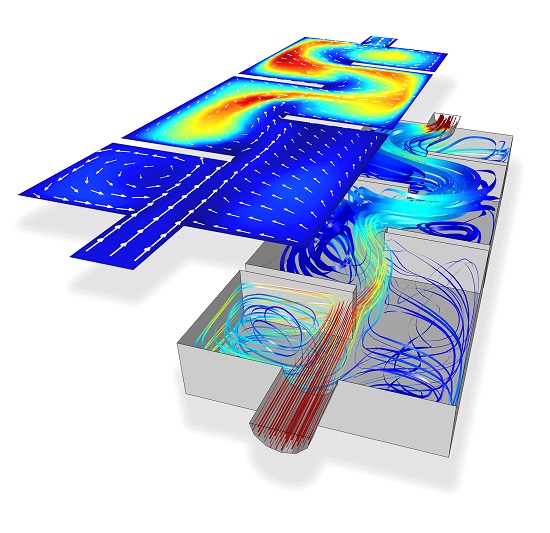
This model computes the structural stresses and deflections on a solar panel due to a turbulent wind load. Different geometries and meshes are used for the fluid and structural problems. The free stream air flow is 15 m/s, and the solar panel is in a regularly spaced array, implying periodic flow boundary conditions.
This example studies a narrow vertical cylinder placed on top of a reservoir filled with water. Because of wall adhesion and surface tension at the air/water interface, water rises through the channel.
Surface tension and wall adhesive forces are often used to transport fluid through microchannels in MEMS devices or to measure, transport and position small amounts of fluid using micropipettes. Multiphase flow through a porous medium and droplets on solid walls are other examples where wall adhesion and surface tension strongly influence the dynamics of the flow.
To model the adhesive forces at the walls correctly, the treatment of the boundary conditions is important. If you fix the velocity to zero on the walls, the interface cannot move along the walls. Instead, you need to allow a non-zero slip velocity and to add a frictional force at the wall. With such a boundary condition, it is possible to explicitly set the contact angle, that is, the angle between the fluid interface and the wall.
The model calculates the pressure field, the velocity field, and the water surface’s shape and position. It uses a level set method, or a phase field method, to track the air/water interface and shows how to add friction and specify the contact angle at the channel walls. The capillary forces dominate over gravity throughout the simulation so that the interface moves upwards during the entire simulation.
The model simulates non-premixed turbulent combustion of syngas (synthesis gas) in a simple round-jet burner.
Syngas is a gas mixture, primarily composed of hydrogen, carbon monoxide and carbon dioxide. The name syngas relates to its use in creating synthetic natural gas. In the model, syngas is fed from a pipe into an open region with a slow co-flow of air. Upon exiting the pipe, the syngas mixes and combusts with the surrounding air in a non-premixed manner. The resulting turbulent flame is attached to the burner head.
The model is solved by combining the Reacting Flow and the Heat Transfer in Fluids interfaces. The turbulent flow in the jet is modeled using the k-ε turbulence model, and the turbulent reactions are modeled using the eddy dissipation model. The resulting velocity, temperature and species mass fractions in the reacting jet are compared to experimental values.
Water treatment basins are used in industrial-scale processes in order to remove bacteria or other contaminants, such as for making water safe to drink.
The Water Treatment Basin application exemplifies the use of apps for modeling turbulent flow and material balances subject to chemical reactions. You can specify the dimensions and orientation of the basin, mixing baffles, and inlet and outlet channels. You can also set the inlet velocity, species concentration, and reaction rate constant in the first-order reaction.
The app solves for the turbulent flow through the basin and presents the resulting flow and concentration fields as well as the space-time, half-life, and pressure drop.
Applying an electric field across a suspension of immiscible liquids may stimulate droplets of the same phase to coalesce. The method known as electrocoalescence has important applications, for instance, in the separation of oil from water.
To model electrocoalescence, you need to solve the Navier-Stokes equations, describing the fluid motion, as well as track the interfaces between the immiscible fluids. In order to include the electric forces, you also have to solve for the electric field. The electric field depends on the position and shape of the water droplets. This complex multiphysics process can readily be set up and solved with COMSOL Multiphysics.
Although initially invented to be used in printers, inkjets have been adopted for other application areas, such as within the life sciences and microelectronics. Simulations can be useful to improve the understanding of the fluid flow and to predict the optimal design of an inkjet for a specific application.
The purpose of this application is to adapt the shape and operation of an inkjet nozzle for a desired droplet size, which depends on the contact angle, surface tension, viscosity, and density of the injected liquid. The results also reveal whether the injected volume breaks up into several droplets before merging into a final droplet at the substrate.
The fluid flow is modeled by the incompressible Navier-Stokes equations together with surface tension, using the level set method to track the fluid interface.
The Ahmed body represents a simplified, ground vehicle geometry of a bluff body type. Its shape is simple enough to allow for accurate flow simulation but retains some important practical features relevant to automobile bodies. This model describes how to calculate the turbulent flow field around a simple car-like geometry using the Turbulent Flow, k-epsilon interface. Detailed instructions guide you through the different steps of the modeling process in COMSOL Multiphysics.
In general, there are two classes of ventilation: mixing ventilation and displacement ventilation. In displacement ventilation, air enters a room at the floor level and displaces warmer air to achieve the desired temperature. Heating sources in the room can include running electronic devices, or inlet jets of warm air. A potential issue with the displacement ventilation approach is that significant temperature variation and strong stratification may arise.
The model investigates the performance of a displacement ventilation system. The flow is modeled using the Non-Isothermal Turbulent Flow, k-omega Model interface.
This model simulates the flow around an inclined NACA 0012 airfoil at different angles of attack using the SST turbulence model. The results show good agreement with the experimental lift data of Ladson and the pressure data of Gregory and O’Reilly.