Image made using the COMSOL Multiphysics® software and is provided courtesy of COMSOL.
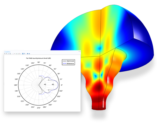
A horn originally had the shape of an axisymmetric cone with a straight boundary. This is optimized with respect to the far-field sound pressure level.
The Optimization Module is an add-on package that you can use in conjunction with any existing COMSOL Multiphysics Product. Once you have created a COMSOL Multiphysics model of your product or process, you always want to improve on your design. This involves four steps. First, you define your objective function – a figure of merit that describes your system. Second, you define a set of design variables – the inputs to the model that you would like to change. Third, you define a set of constraints, bounds on your design variables, or operating conditions that need to be satisfied. Last, you use the Optimization Module to improve your design by changing the design variables, while satisfying your constraints. The Optimization Module is a general interface for defining objective functions, specifying design variables, and setting up these constraints. Any model input, whether it be geometric dimensions, part shapes, material properties, or material distribution, can be treated as a design variable, and any model output can be used to define the objective function. It can be used throughout the COMSOL Multiphysics product family and can be combined with the LiveLink™ add-on products to optimize a geometric dimension in a third-party CAD program.
This presentation shows how to use the Optimization Module to fit a material model curve to experimental data. It is based on the hyperelastic Mooney-Rivlin material model example given in the Structural Mechanics users guide.
The goal with this application is to explain experimental electrochemical impedance spectroscopy (EIS) measurements and to show how you can use a simulation app along with measurements to estimate the properties of lithium-ion batteries. The Lithium-Ion Battery Impedance app takes measurements from an EIS experiment and uses them as inputs. It then simulates these measurements and runs a parameter estimation based on the experimental data.
The control parameters are the exchange current density, the resistivity of the solid electrolyte interface on the particles, the double-layer capacitance of NCA, the double-layer capacitance of the carbon support in the positive electrode, and the diffusivity of the lithium ion in the positive electrode. Fitting is done to the measured impedance of the positive electrode at frequencies ranging from 10 mHz to 1 kHz.
Imagine that you are designing a light-weight mountain bike frame that should fit in a box of a certain size and should weigh no more than 8 kg. Given that you know the loads on the bike, you can achieve this by distributing the available material while making sure that the stiffness of the frame is at a maximum. This way you have formulated the topology optimization of the frame as a material distribution problem.
This model demonstrates how you can apply the SIMP model (Solid Isotropic Material with Penalization) for structural topology optimization with COMSOL Multiphysics.
The particular model solves the problem of finding the optimal distribution of a given amount of material forming an L-shaped frame. The optimality criterion is a minimum compliance for the load case where the frame’s upper boundary is fixed and a downward load is applied along its right end.
The radial stress component in an axially symmetric and homogeneous flywheel of constant thickness exhibits a sharp peak near the inner radius. From there, it decreases monotonously until it reaches zero at the flywheel’s outer rim. The uneven stress distribution reveals a design that does not make optimal use of the material available.
Given specified flywheel mass and moment of inertia, this model solves the problem of finding the optimal thickness profile with respect to the objective of obtaining a radial stress distribution that is as even as possible.
The resulting maximum stress, which occurs in the radial direction at the inner radius, is roughly 40% less for the optimized profile compared to the flat flywheel.
A demonstration of topology optimization using the Structural Mechanics Module and the Optimization Module. Three classical models are shown, the loaded knee, the Michell truss structure, and MBB beam. The optimization method is based on using the SIMPS approach to recast the original combinatorial optimization problem into a continuous optimization problem.
Topology optimization of the Navier-Stokes equations is encountered in different branches and applications, such as in the design of ventilation systems for cars. A common technique applicable to such problems is to let the distribution of porous material vary continuously.
In this model, the objective is to find the optimal distribution of a porous material in a microchannel such that the horizontal velocity component at the center of the channel is minimized.