Image made using the COMSOL Multiphysics® software and is provided courtesy of COMSOL.
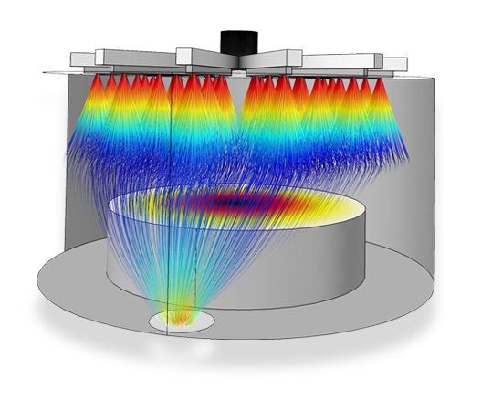
Particles are injected from a system of injection nozzles into a CVD chamber with a cone angle of 15 degrees. Initially they have enough inertia to follow their original trajectory but ultimately the drag force takes over and the particles begin to follow the background gas out of the exhaust port.
The Particle Tracing Module extends the functionality of the COMSOL environment for computing the trajectory of particles in a fluid or electromagnetic field, including particle-particle, fluid-particle, and particle-field interactions. You can seamlessly combine any application-specific module with the Particle Tracing Module for computing the fields that drive particle motion. Particles can have mass or be mass-less. The movement is governed by either the Newtonian, Lagrangian, or Hamiltonian formulations from classical mechanics. Boundary conditions can be imposed on the particles on the walls of the geometry to allow particles to freeze, stick, bounce, disappear, or reflect diffusely. User-defined wall conditions may also be specified, where the post collision particle velocity is typically a function of the incoming particle velocity and the wall normal vector. Secondary particles released when an incoming particle strikes a wall can be included. The number of secondary particles and their velocity distribution function can be functions of the primary particle velocity and the wall geometry. Particles can also stick to the wall according to an arbitrary expression or a sticking probability. Additional dependent variables can be added to the model which allows you to compute quantities like particle mass, temperature, or spin.
Particles can be released on boundaries and domains uniformly, according to the underlying mesh, as defined by a grid or according to an arbitrary expression. A wide range of predefined forces is available to describe specifically how the particles interact with the fields. You can then add arbitrary forces as defined by a suitable expression. It is also possible to model the two-way interaction between the particles and the fields (particle-field interaction), as well as the interaction of particles between each other (particle-particle interaction).
Dielectrophoresis (DEP) occurs when a force is exerted on a dielectric particle as it is subjected to a nonuniform electric field. DEP has many applications in the field of biomedical devices used for biosensors, diagnostics, particle manipulation and filtration (sorting), particle assembly, and more.
The DEP force is sensitive to the size, shape, and dielectric properties of the particles. This allows DEP to be used to separate different kinds of particles, such as various kinds of cells from a mixture. The Red Blood Cell Separation application shows how red blood cells can be selectively filtered from a blood sample in order to isolate red blood cells from platelets.
In the DEP filter device, the red blood cells, which are larger than the platelets, feel a larger force and are thereby deflected more. The two outlets are arranged so that the top outlet catches undeflected particles and only particles that have been deflected can exit from the lower outlet.
The app allows you to vary characteristics of the red blood cells and platelets, as well as the electric field.
In static mixers, also called motionless or in-line mixers, a fluid is pumped through a pipe containing stationary blades. This mixing technique is particularly well suited for laminar flow mixing because it generates only small pressure losses in this flow regime. This example studies the flow in a twisted-blade static mixer. It evaluates the mixing performance by calculating the trajectory of suspended particles through the mixer. The model uses the Laminar Flow and Particle Tracing for Fluid Flow interfaces.
When modeling the propagation of charged particle beams at high currents, the space charge force generated by the beam significantly affects the trajectories of the charged particles. Perturbations to these trajectories, in turn, affect the space charge distribution.
The Charged Particle Tracing interface can use an iterative procedure to efficiently compute the strongly coupled particle trajectories and electric field for systems operating under steady-state conditions. Such a procedure reduces the required number of model particles by several orders of magnitude, compared to methods based on explicit modeling of Coulomb interactions between the beam particles. A mesh refinement study confirms that the solution agrees with the analytical expression for the shape of a nonrelativistic, paraxial beam envelope.
In static mixers, a fluid is pumped through a pipe containing stationary mixing blades. This mixing technique is well suited for laminar flow mixing, because it generates only small pressure losses in this flow regime. When a fluid is pumped through the channel, the alternating directions of the cross-sectional blades mix the fluid as it passes along the length of the channel. The static mixing technique allows for precise control over the amount of mixing that takes place throughout the process. However, the performance of the mixer can vary greatly, depending on its geometry.
The Laminar Static Particle Mixer Designer app computes the fluid velocity and pressure field in a static mixer, as well as the trajectories of particles that are carried by the fluid. Because the particles have mass, they do not follow the fluid velocity streamlines exactly, causing some particles to hit the mixing blades.
The example app computes the transmission probability of particles in the mixer. It also evaluates the index of dispersion, which is a measurement of the uniformity with which different species of particles are mixed together.
A charge exchange cell consists of a region of gas at an elevated pressure within a vacuum chamber. When an ion beam interacts with the higher-density gas, the ions undergo charge exchange reactions with the gas, creating energetic neutral particles. It is likely that only a fraction of the beam ions will undergo charge exchange reactions. Therefore, in order to neutralize the beam, a pair of charged deflecting plates are positioned outside the cell. In this way, an energetic neutral source can be produced.
The Charge Exchange Cell Simulator app simulates the interaction of a proton beam with a charge exchange cell containing neutral argon. User inputs include several geometric parameters for the gas cell and vacuum chamber, beam properties, and the properties of the charged plates that are used to deflect the remaining ions.
The simulation app computes the efficiency of the charge exchange cell, measured as the fraction of ions that are neutralized, and records statistics about the different types of collisions that occur.
This model computes the trajectory of an ion in a uniform magnetic field using the Newtonian, Lagrangian and Hamiltonian formulations available in the Mathematical Particle Tracing interface.
Transport which is purely diffusive in nature can be modeled using a Brownian force. This model shows how to add such a force in the Particle Tracing for Fluid Flow physics interface. Particle diffusion in a fluid is modeled with the diffusion equation and the Particle Tracing for Fluid flow interfaces and the results are compared.
This model demonstrates the use of optical tracing for studying optically large gradient-index structures with anisotropic optical properties. Additionally, the model introduces a smoothing technique for handling discontinuities of refractive index on curved surfaces, which are typical in conventional optical devices such as lenses.
This tutorial model shows how to add customized particle-particle interaction forces. In this example the gravitational force between 2500 stars in a galaxy is modeled. The galaxy initially rotates as a rigid body, then begins to change shape due to gravitational forces.